on
Portfolio Simulator
This document is intended to help those interested in venture capital reason about expected fund-level returns. All multiples are net to LPs (i.e. after fees and 20 % carry) unless noted. I wrote this originally in 2023, and updated it in April 2025 with about 60 min of vibe coding.
I took data from this 2020 report (page 14), and filtered it for the 10 year period between 2004 and 2013. I chose that period because the vintages surrounding the internet bubble show unusually high volatility, and discarded years closer to 2020 given that it takes about 7 years for the TVPI to stabilize. I also used Angel List to estimate some of the higher percentiles, although the time period for this data is unclear.
Cambridge Associates 10-yr TVPI (2004-2013)
| Vintage | Pooled | Mean | Median | Upper Q | Lower Q | Funds |
| ------- | ------ | ---- | ------ | ------- | ------- | ----- |
| 2004    | 1.69   | 1.72 | 1.2    | 1.82    | 0.82    | 63    |
| 2005    | 1.68   | 1.66 | 1.41   | 2.07    | 0.91    | 61    |
| 2006    | 1.69   | 1.56 | 1.59   | 1.95    | 0.75    | 78    |
| 2007    | 2.29   | 2.38 | 1.76   | 2.93    | 1.31    | 68    |
| 2008    | 1.77   | 1.71 | 1.4    | 2.21    | 1.09    | 64    |
| 2009    | 2.1    | 2.12 | 1.75   | 2.46    | 1.3     | 23    |
| 2010    | 3.21   | 2.8  | 2.12   | 3.41    | 1.41    | 48    |
| 2011    | 2.48   | 2.26 | 1.9    | 2.71    | 1.39    | 44    |
| 2012    | 2.21   | 2.48 | 1.73   | 2.37    | 1.35    | 55    |
| 2013    | 2.02   | 2.01 | 1.81   | 2.26    | 1.34    | 59    |
| Average | 2.11   | 2.07 | 1.67   | 2.42    | 1.17    | 56    |
Angel List Fund Performance Calculator (April 2025)
| Percentile | Net IRR |
| ---------- | ------- |
| 90th       | 35%     |
| 95th       | 40%     |
| 99th       | 55%     |
Core assumptions
- Fund size $50 M — prototypical seed/Series A vehicle
(Fund size is implicit; all multiples are net-to-LP.) - Fee load 15 % lifetime (≈ 2 % per year for 7-8 years, charged up-front)
- Carry 20 % GP promote on profits after fees
- Initial cheques 22 equal-sized first investments, no follow-ons — keeps the portfolio math clean
- Deal-outcome model
- 55 % outright zeros (0×)
- 45 % survivors drawn from LogNormal (μ = 1.10, σ = 1.40), capped at 200×
↳ Continuous returns smooth the histogram and anchor the 95 th percentile near ~6×.
- Capital calls 25 % of committed capital in each of years 0-3 — mirrors common pacing
- Exit timing Each company realises its full value in a single lump-sum exit uniformly between years 4-10 — spreads cash flows for a realistic IRR profile
- IRR calculation Exact cash-flow schedule solved with
numpy_financial.irr— no midpoint shortcuts - Reproducibility Fixed NumPy RNG seed 2025; 3 500 simulated funds — rerun and you’ll get identical tables and plots
Simulated Results
| Percentile | Sim TVPI | Sim IRR % |
| ---------- | -------- | --------- |
| 25th       | 1.45     | 5.6       |
| 50th       | 2.09     | 12        |
| 75th       | 3.16     | 20.7      |
| 90th       | 4.6      | 30.7      |
| 95th       | 5.85     | 38.6      |
| 99th       | 8.31     | 55.8      |
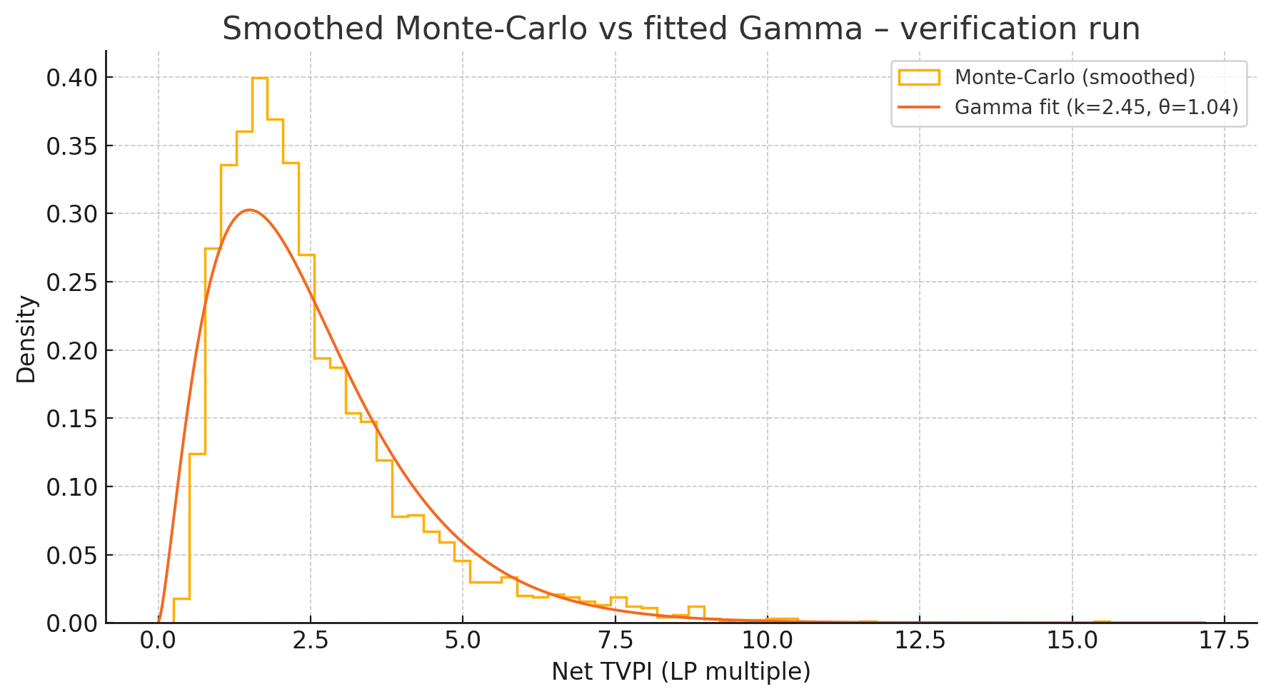
We fit a Gamma distribution to the Monte-Carlo TVPI sample after the simulation finishes. Overlaying this analytic curve serves two purposes: first, it provides a quick visual check that the simulated histogram has the expected shape, and second, it gives readers a neat closed-form PDF and CDF they can drop into their own spreadsheets without rerunning thousands of Monte-Carlo draws.
Code
"""
Smoothed Venture-Fund Monte-Carlo Simulator
==========================================

This script generates a continuous, log-normal–based deal-level simulation
that matches target fund-level TVPI percentiles, then:

  • Computes IRRs with an explicit cash-flow schedule
  • Prints a Markdown-formatted percentile table (TVPI + IRR)
  • Plots the Monte-Carlo histogram with a moment-matched Gamma overlay

Best-fit parameters were hand-picked from a prior grid search and are
hard-coded here, so there is **no grid search** on execution.

Author : Ivan Bercovich (April 2025)
License: MIT
"""

# --------------------------------------------------------------------------- #
# 1. Imports
# --------------------------------------------------------------------------- #
import numpy as np
import numpy_financial as npf        # IRR solver
import pandas as pd
import matplotlib.pyplot as plt
import math
import tabulate
from textwrap import indent

# NB: matplotlib uses your active backend; no style tweaks applied to keep
#     portability high.

# --------------------------------------------------------------------------- #
# 2. Global settings (purely reproducibility + model inputs)
# --------------------------------------------------------------------------- #
SEED       = 2025          # deterministic RNG seed
N_FUNDS    = 3_500         # Monte-Carlo fund draws
N_INVEST   = 22            # equal-size first cheques (no follow-on)

# ---------- Deal-outcome model ---------- #
# “Fail” cheques return 0×.
# “Survivors” follow a single *log-normal* distribution, truncated to cap
# pathological outliers (>200× is exceedingly rare in seed funds).
P_FAIL     = 0.55          # probability a cheque is a total write-off
MU_LN      = 1.10          # log-mean  (in ln-space) of survivor multiples
SIGMA_LN   = 1.40          # log-std-dev of survivor multiples
MAX_MULT   = 200.0         # hard cap on extreme successes

# ---------- Fund economics ---------- #
MGMT_FEE   = 0.15          # lifetime management fees (15 % of committed)
CARRY      = 0.20          # GP carry on profits (standard “80 / 20” split)

# ---------- Exit-timing logic ---------- #
EXIT_YEAR_MIN = 4          # earliest exit
EXIT_YEAR_MAX = 10         # latest exit
# A single lump-sum distribution is drawn uniformly in [4, 10].

# ---------- Targets for reference ---------- #
TARGET_TVPI  = np.array([1.25, 2.0, 2.75, 5.0, 6.5, 8.0])    # 25–99 th
PERCENTILES  = [25, 50, 75, 90, 95, 99]

# --------------------------------------------------------------------------- #
# 3. Helper functions
# --------------------------------------------------------------------------- #
def draw_survivor_returns(size: int, rng: np.random.Generator) -> np.ndarray:
    """
    Draw `size` log-normal multiples and cap them at `MAX_MULT`.

    Parameters
    ----------
    size : int
        Number of survivor cheques to simulate.
    rng  : np.random.Generator
        Numpy RNG instance for reproducibility.

    Returns
    -------
    np.ndarray
        1-D float array of length `size`, each ≥ 0.01 × and ≤ MAX_MULT ×.
    """
    draws = rng.lognormal(MU_LN, SIGMA_LN, size)
    return np.clip(draws, 0.01, MAX_MULT)


def simulate_fund_tvpi(rng: np.random.Generator) -> float:
    """
    Simulate one fund’s **net-to-LP TVPI**.

    Steps
    -----
    1.  Sample failures vs survivors for each of `N_INVEST` cheques.
    2.  Draw continuous survivor returns.
    3.  Take the arithmetic mean ⇒ gross TVPI (all cheques equal size).
    4.  Convert gross ⇒ net by subtracting fees and applying carry.

    Returns
    -------
    float
        Net TVPI (multiple of distributed / committed capital).
    """
    # 1) Boolean mask of failures
    fails = rng.random(N_INVEST) < P_FAIL
    n_survivors = (~fails).sum()

    # 2) Continuous survivor multiples
    survivor_mults = (
        draw_survivor_returns(n_survivors, rng) if n_survivors else np.array([])
    )

    # 3) Portfolio gross multiple (simple mean; failures contribute zero)
    gross_tvpi = survivor_mults.sum() / N_INVEST

    # 4) Net to LPs: LP capital is reduced by mgmt. fee, and GP takes 20 % carry
    net_tvpi = (1 - MGMT_FEE) * (1 + (1 - CARRY) * (gross_tvpi - 1))
    return net_tvpi


def fund_irr(tvpi: float, exit_year: int) -> float:
    """
    Compute an internal rate of return given:

      • `tvpi`   – net multiple (already net of fees & carry)
      • `exit_year` – year in which *all* gains are realised

    Capital calls: –25 % in each of years 0, 1, 2, 3.
    """
    calls = [-0.25] * 4                         # negative cash flows
    cfs   = calls + [0] * (exit_year - 3) + [tvpi]
    return npf.irr(cfs)         # returns decimal (e.g. 0.15 ⇒ 15 % IRR)


def markdown_table(df: pd.DataFrame) -> str:
    """Return a DataFrame rendered as GitHub-flavoured Markdown."""
    return df.to_markdown(index=False, tablefmt="github")

# --------------------------------------------------------------------------- #
# 4. Monte-Carlo simulation
# --------------------------------------------------------------------------- #
rng = np.random.default_rng(SEED)

# ---- Run the fund loop ---- #
tvpi_mc = np.array([simulate_fund_tvpi(rng) for _ in range(N_FUNDS)])

# ---- Assign a random exit year per fund ---- #
exit_years = rng.integers(EXIT_YEAR_MIN, EXIT_YEAR_MAX + 1, N_FUNDS)
irr_mc     = np.array(
    [fund_irr(m, yr) for m, yr in zip(tvpi_mc, exit_years)]
) * 100    # convert to %

# --------------------------------------------------------------------------- #
# 5. Summarise results in Markdown
# --------------------------------------------------------------------------- #
summary_df = pd.DataFrame({
    "Percentile":  [f"{p}th" for p in PERCENTILES],
    "Target TVPI": TARGET_TVPI,
    "Sim TVPI":    np.round(np.percentile(tvpi_mc,  PERCENTILES), 2),
    "Sim IRR %":   np.round(np.percentile(irr_mc,   PERCENTILES), 1),
})

print("\n### Monte-Carlo Results (Markdown table)\n")
print(markdown_table(summary_df))

# --------------------------------------------------------------------------- #
# 6. Fit a Gamma distribution for visual overlay
# --------------------------------------------------------------------------- #
mu, var = tvpi_mc.mean(), tvpi_mc.var()
shape_g = mu**2 / var          # k
scale_g = var / mu             # θ

# Analytical Gamma PDF for plotting
x = np.linspace(0, tvpi_mc.max() * 1.1, 500)
pdf_gamma = (
    x ** (shape_g - 1) * np.exp(-x / scale_g)
) / (math.gamma(shape_g) * scale_g**shape_g)

# --------------------------------------------------------------------------- #
# 7. Plot histogram + Gamma overlay
# --------------------------------------------------------------------------- #
plt.figure(figsize=(9, 5))
plt.hist(
    tvpi_mc,
    bins=60,
    density=True,
    histtype="step",
    lw=1.25,
    label="Monte-Carlo (smoothed)",
)
plt.plot(
    x,
    pdf_gamma,
    lw=1.4,
    label=f"Gamma fit (k={shape_g:.2f}, θ={scale_g:.2f})",
)
plt.xlabel("Net TVPI (LP multiple)")
plt.ylabel("Density")
plt.title("Smoothed Monte-Carlo vs fitted Gamma")
plt.legend()
plt.tight_layout()
plt.show()

# --------------------------------------------------------------------------- #
# 8. Print key simulation settings (optional provenance block)
# --------------------------------------------------------------------------- #
print("\n---  Simulation parameters  -------------------------------------------")
print(
    indent(
        f"""
    Funds simulated        : {N_FUNDS}
    Cheques per fund       : {N_INVEST}
    Failure probability    : {P_FAIL:.0%}
    Survivor log-normal μ  : {MU_LN:.2f}
    Survivor log-normal σ  : {SIGMA_LN:.2f}
    Management fee (lifetime) : {MGMT_FEE:.0%}
    Carry                   : {CARRY:.0%}
    Exit year distribution  : Uniform [{EXIT_YEAR_MIN}, {EXIT_YEAR_MAX}]
    RNG seed               : {SEED}
""".strip(),
        prefix="  ",
    )
)